Analysis of Experiment 2
Last updated: 2021-12-10
Checks: 7 0
Knit directory: social_immunity/
This reproducible R Markdown analysis was created with workflowr (version 1.6.2). The Checks tab describes the reproducibility checks that were applied when the results were created. The Past versions tab lists the development history.
Great! Since the R Markdown file has been committed to the Git repository, you know the exact version of the code that produced these results.
Great job! The global environment was empty. Objects defined in the global environment can affect the analysis in your R Markdown file in unknown ways. For reproduciblity it’s best to always run the code in an empty environment.
The command set.seed(20191017) was run prior to running the code in the R Markdown file. Setting a seed ensures that any results that rely on randomness, e.g. subsampling or permutations, are reproducible.
Great job! Recording the operating system, R version, and package versions is critical for reproducibility.
Nice! There were no cached chunks for this analysis, so you can be confident that you successfully produced the results during this run.
Great job! Using relative paths to the files within your workflowr project makes it easier to run your code on other machines.
These are the previous versions of the repository in which changes were made to the R Markdown (analysis/experiment2.Rmd) and HTML (docs/experiment2.html) files. If you’ve configured a remote Git repository (see ?wflow_git_remote), click on the hyperlinks in the table below to view the files as they were in that past version.
| File | Version | Author | Date | Message |
|---|---|---|---|---|
| Rmd | 5f0a4d8 | lukeholman | 2021-12-10 | wflow_publish(“analysis/experiment2.Rmd”) |
| html | fbfbba5 | lukeholman | 2021-12-10 | Build site. |
| Rmd | 0a2588c | lukeholman | 2021-12-10 | wflow_publish(“analysis/experiment2.Rmd”) |
| html | fbfc820 | lukeholman | 2021-04-28 | Build site. |
| Rmd | be8266d | lukeholman | 2021-04-28 | wflow_publish("analysis/*") |
| html | af7a3ea | lukeholman | 2021-04-27 | Build site. |
| html | 3e419d1 | lukeholman | 2021-04-27 | Build site. |
| Rmd | 43d5c2f | lukeholman | 2021-04-27 | Behav Ecol version |
| html | 5bd1725 | lukeholman | 2021-01-12 | Build site. |
| Rmd | 62a950c | lukeholman | 2021-01-12 | mostly ready |
| html | 9ebe5df | lukeholman | 2021-01-12 | Build site. |
| Rmd | 9c79d22 | lukeholman | 2021-01-12 | mostly ready |
| html | 939ecd0 | lukeholman | 2021-01-11 | Build site. |
| Rmd | 78386bb | lukeholman | 2021-01-11 | tweaks 2021 |
| html | eeb5a09 | lukeholman | 2020-11-30 | Build site. |
| Rmd | 7aa69df | lukeholman | 2020-11-30 | Added simple models |
| html | 7131f65 | lukeholman | 2020-08-21 | Build site. |
| Rmd | c80c978 | lukeholman | 2020-08-21 | Fix summarise() warnings |
| html | 4f23e70 | lukeholman | 2020-08-21 | Build site. |
| Rmd | c5c8df4 | lukeholman | 2020-08-21 | Minor fixes |
| html | 1bea769 | lukeholman | 2020-08-21 | Build site. |
| Rmd | d1dade3 | lukeholman | 2020-08-21 | added supp material |
| html | 7bf607f | lukeholman | 2020-05-02 | Build site. |
| Rmd | 83fa522 | lukeholman | 2020-05-02 | tweaks |
| html | 3df58c2 | lukeholman | 2020-05-02 | Build site. |
| html | 2994a41 | lukeholman | 2020-05-02 | Build site. |
| html | d166566 | lukeholman | 2020-05-02 | Build site. |
| html | fedef8f | lukeholman | 2020-05-02 | Build site. |
| Rmd | 6c7445f | lukeholman | 2020-05-02 | tweak colours |
| html | 4cb9bc1 | lukeholman | 2020-05-02 | Build site. |
| Rmd | 14377be | lukeholman | 2020-05-02 | tweak colours |
| html | 14377be | lukeholman | 2020-05-02 | tweak colours |
| html | fa8c179 | lukeholman | 2020-05-02 | Build site. |
| Rmd | f188968 | lukeholman | 2020-05-02 | tweak colours |
| html | f188968 | lukeholman | 2020-05-02 | tweak colours |
| html | 2227713 | lukeholman | 2020-05-02 | Build site. |
| Rmd | f97baee | lukeholman | 2020-05-02 | Lots of formatting changes |
| html | f97baee | lukeholman | 2020-05-02 | Lots of formatting changes |
| html | 1c9a1c3 | lukeholman | 2020-05-02 | Build site. |
| Rmd | 3d21d6a | lukeholman | 2020-05-02 | wflow_publish("*", republish = T) |
| html | 3d21d6a | lukeholman | 2020-05-02 | wflow_publish("*", republish = T) |
| html | 93c487a | lukeholman | 2020-04-30 | Build site. |
| html | 5c45197 | lukeholman | 2020-04-30 | Build site. |
| html | 4bd75dc | lukeholman | 2020-04-30 | Build site. |
| Rmd | 12953af | lukeholman | 2020-04-30 | test new theme |
| html | 12953af | lukeholman | 2020-04-30 | test new theme |
| html | d6437a5 | lukeholman | 2020-04-25 | Build site. |
| html | e58e720 | lukeholman | 2020-04-25 | Build site. |
| html | 71b6160 | lukeholman | 2020-04-25 | Build site. |
| Rmd | 76a317d | lukeholman | 2020-04-25 | tweaks |
| html | 2235ae4 | lukeholman | 2020-04-25 | Build site. |
| Rmd | 99649a7 | lukeholman | 2020-04-25 | tweaks |
| html | 99649a7 | lukeholman | 2020-04-25 | tweaks |
| html | 0ede6e3 | lukeholman | 2020-04-24 | Build site. |
| Rmd | a1f8dc2 | lukeholman | 2020-04-24 | tweaks |
| html | 8c3b471 | lukeholman | 2020-04-21 | Build site. |
| Rmd | 1ce9e19 | lukeholman | 2020-04-21 | First commit 2020 |
| html | 1ce9e19 | lukeholman | 2020-04-21 | First commit 2020 |
| Rmd | aae65cf | lukeholman | 2019-10-17 | First commit |
| html | aae65cf | lukeholman | 2019-10-17 | First commit |
Load data and R packages
# All but 1 of these packages can be easily installed from CRAN.
# However it was harder to install the showtext package. On Mac, I did this:
# installed 'homebrew' using Terminal: ruby -e "$(curl -fsSL https://raw.githubusercontent.com/Homebrew/install/master/install)"
# installed 'libpng' using Terminal: brew install libpng
# installed 'showtext' in R using: devtools::install_github("yixuan/showtext")
library(showtext)

library(brms)
library(lme4)
library(bayesplot)
library(tidyverse)
library(gridExtra)
library(kableExtra)
library(bayestestR)
library(tidybayes)
library(cowplot)
library(car)
source("code/helper_functions.R")

# set up nice font for figure
nice_font <- "Lora"
font_add_google(name = nice_font, family = nice_font, regular.wt = 400, bold.wt = 700)
showtext_auto()

exp2_treatments <- c("Ringers", "LPS")

durations <- read_csv("data/data_collection_sheets/experiment_durations.csv") %>%
  filter(experiment == 2) %>% select(-experiment)

outcome_tally <- read_csv(file = "data/clean_data/experiment_2_outcome_tally.csv") %>%
  mutate(
    outcome = str_replace_all(outcome, "Stayed inside the hive", "Stayed inside"),
    outcome = str_replace_all(outcome, "Left of own volition", "Left voluntarily"),
    outcome = factor(outcome, levels = c("Stayed inside", "Left voluntarily", "Forced out")),
         treatment = str_replace_all(treatment, "Ringer CHC", "Ringers"),
         treatment = str_replace_all(treatment, "LPS CHC", "LPS"),
         treatment = factor(treatment, levels = exp2_treatments))

# Re-formatted version of the same data, where each row is an individual bee. We need this format to run the brms model.
data_for_categorical_model <- outcome_tally %>%
  mutate(id = 1:n()) %>%
  split(.$id) %>%
  map(function(x){
    if(x$n[1] == 0) return(NULL)
    data.frame(
      treatment = x$treatment[1],
      hive = x$hive[1],
      colour = x$colour[1],
      outcome = rep(x$outcome[1], x$n))
  }) %>% do.call("rbind", .) %>% as_tibble() %>%
  arrange(hive, treatment) %>%
  mutate(outcome_numeric = as.numeric(outcome),
         hive = as.character(hive),
         treatment = factor(treatment, levels = exp2_treatments)) %>%
  left_join(durations, by = "hive") %>%
  mutate(hive = C(factor(hive), sum))  # use "sum coding" for hive, since there is no obvious reference level
Inspect the raw data
Click the three tabs to see each table.
Sample sizes by treatment
sample_sizes <- data_for_categorical_model %>%
  group_by(treatment) %>%
  summarise(n = n(), .groups = "drop")

sample_sizes %>%
kable() %>% kable_styling(full_width = FALSE)| treatment | n |
|---|---|
| Ringers | 294 |
| LPS | 291 |
Sample sizes by treatment and hive
data_for_categorical_model %>%
  group_by(hive, treatment) %>%
  summarise(n = n(), .groups = "drop") %>%
  spread(treatment, n) %>%
kable() %>% kable_styling(full_width = FALSE)| hive | Ringers | LPS |
|---|---|---|
| Arts | 70 | 68 |
| Garden | 75 | 75 |
| Skylab | 99 | 100 |
| Zoology | 50 | 48 |
Oberved outcomes
outcome_tally %>%
  select(-colour) %>%
  spread(outcome, n) %>%
kable(digits = 3) %>% kable_styling(full_width = FALSE) | hive | treatment | Stayed inside | Left voluntarily | Forced out |
|---|---|---|---|---|
| Arts | Ringers | 64 | 5 | 1 |
| Arts | LPS | 56 | 5 | 7 |
| Garden | Ringers | 73 | 2 | 0 |
| Garden | LPS | 70 | 2 | 3 |
| Skylab | Ringers | 97 | 1 | 1 |
| Skylab | LPS | 93 | 2 | 5 |
| Zoology | Ringers | 42 | 2 | 6 |
| Zoology | LPS | 38 | 4 | 6 |
Preliminary GLMM
The multinomial model below is not commonly used, though we believe it is the right choice for this particular experiment (e.g. because it can model a three-item categorical response variable, and it can incorporate priors). However during peer review, we were asked whether the results were similar when using standard statistical methods. To address this question, we here present a frequentist Generalised Linear Mixed Model (GLMM; using lme4::glmer), which tests the null hypothesis that the proportion of bees exiting the hive (i.e. the proportion leaving voluntarily plus those that were forced out) is equal between treatment groups and hives.
The model results are similar to those from the multinomial model: bees treated with the CHCs from LPS-treated nestmates left the hive more often than controls, and there was variation between hives in the proportion of bees leaving.
glmm_data <- outcome_tally %>%
  group_by(hive, treatment, outcome) %>%
  summarise(n = sum(n)) %>%
  mutate(left = ifelse(outcome == "Stayed inside", "stayed_inside" ,"left_hive")) %>%
  group_by(hive, treatment, left) %>%
  summarise(n = sum(n)) %>%
  spread(left, n)

simple_model <- glmer(
    cbind(left_hive, stayed_inside) ~ treatment + (1 | hive),
    data = glmm_data,
    family = "binomial")
summary(simple_model)
Generalized linear mixed model fit by maximum likelihood (Laplace Approximation) ['glmerMod']
Family: binomial ( logit )
Formula: cbind(left_hive, stayed_inside) ~ treatment + (1 | hive)
Data: glmm_data
AIC BIC logLik deviance df.resid
45.6 45.9 -19.8 39.6 5
Scaled residuals:
Min 1Q Median 3Q Max
-0.77963 -0.28362 -0.05464 0.09864 0.97893
Random effects:
Groups Name Variance Std.Dev.
hive (Intercept) 0.3975 0.6305
Number of obs: 8, groups: hive, 4
Fixed effects:
Estimate Std. Error z value Pr(>|z|)
(Intercept) -2.7789 0.4022 -6.909 4.87e-12 ***
treatmentLPS 0.7410 0.3062 2.420 0.0155 *
---
Signif. codes: 0 '***' 0.001 '**' 0.01 '*' 0.05 '.' 0.1 ' ' 1
Correlation of Fixed Effects:
(Intr)
treatmntLPS -0.488Baysian multinomial model
Fit the model
Fit the multinomial logistic models, with a 3-item response variable describing what happened to each bee introduced to the hive: stayed inside, left voluntarily, or forced out by the other workers.
if(!file.exists("output/exp2_model.rds")){

  prior <- c(set_prior("normal(0, 3)", class = "b", dpar = "mu2"),
             set_prior("normal(0, 3)", class = "b", dpar = "mu3"),
             set_prior("normal(0, 1)", class = "sd", dpar = "mu2", group = "hive"),
             set_prior("normal(0, 1)", class = "sd", dpar = "mu3", group = "hive"))

  exp2_model <- brm(
    outcome_numeric ~ treatment + (1 | hive),
    data = data_for_categorical_model,
    prior = prior,
    family = "categorical",
    control = list(adapt_delta = 0.99),
    chains = 4, cores = 1, iter = 5000, seed = 1)

  saveRDS(exp2_model, "output/exp2_model.rds")
}

exp2_model <- readRDS("output/exp2_model.rds")
Posterior predictive check
This plot shows ten predictions from the posterior (pale blue) as well as the original data (dark blue), for the three categorical outcomes (1: stayed inside, 2: left voluntarily, 3: forced out). The predicted number of bees in each outcome category is similar to the real data, illustrating that the model is able to recapitulate the original data fairly closely (a necessary requirement for making inferences from the model).
pp_check(exp2_model, type = "hist", nsamples = 8)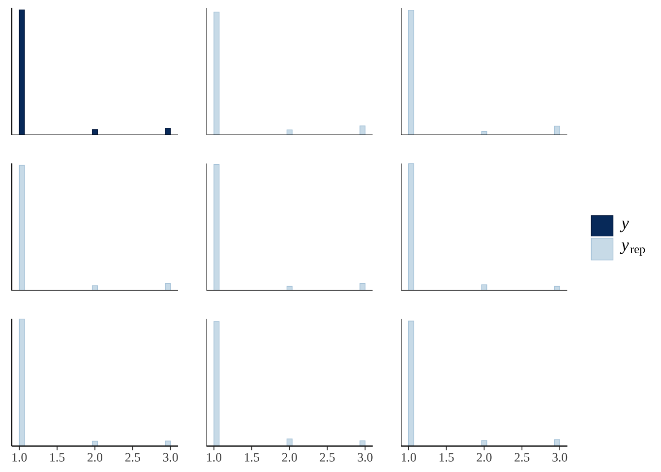
Parameter estimates from the model
Raw output of the treatment + hive model
summary(exp2_model) Family: categorical
Links: mu2 = logit; mu3 = logit
Formula: outcome_numeric ~ treatment + (1 | hive)
Data: data_for_categorical_model (Number of observations: 585)
Samples: 4 chains, each with iter = 5000; warmup = 2500; thin = 1;
total post-warmup samples = 10000
Group-Level Effects:
~hive (Number of levels: 4)
Estimate Est.Error l-95% CI u-95% CI Rhat Bulk_ESS Tail_ESS
sd(mu2_Intercept) 0.76 0.43 0.08 1.78 1.00 2977 2360
sd(mu3_Intercept) 0.89 0.42 0.24 1.90 1.00 2895 2124
Population-Level Effects:
Estimate Est.Error l-95% CI u-95% CI Rhat Bulk_ESS Tail_ESS
mu2_Intercept -3.42 0.55 -4.60 -2.39 1.00 4199 4540
mu3_Intercept -3.65 0.62 -4.96 -2.47 1.00 3805 4780
mu2_treatmentLPS 0.35 0.44 -0.51 1.21 1.00 10040 7134
mu3_treatmentLPS 1.08 0.43 0.27 1.96 1.00 9634 6392
Samples were drawn using sampling(NUTS). For each parameter, Bulk_ESS
and Tail_ESS are effective sample size measures, and Rhat is the potential
scale reduction factor on split chains (at convergence, Rhat = 1).Formatted brms output for Table S3
The code chunk below wrangles the raw output of the summary() function for brms models into a more readable table of results, and also adds ‘Bayesian p-values’ (i.e. the posterior probability that the true effect size has the same sign as the reported effect).
Table S3: Table summarising the posterior estimates of each fixed effect in the model of Experiment 2. This was a multinomial model with three possible outcomes (Stayed inside, Left voluntarily, or Forced out), and so there are two parameter estimates for each predictor in the model. ‘Treatment’ is a fixed factor with two levels, and the effect of LPS shown here is expressed relative to the ‘Ringers’ treatment. The PP column gives the posterior probability that the true effect size is opposite in sign to what is reported in the Estimate column, similarly to a \(p\)-value.
tableS3 <- get_fixed_effects_with_p_values(exp2_model) %>%
  mutate(mu = map_chr(str_extract_all(Parameter, "mu[:digit:]"), ~ .x[1]),
         Parameter = str_remove_all(Parameter, "mu[:digit:]_"),
         Parameter = str_replace_all(Parameter, "treatment", "Treatment: ")) %>%
  arrange(mu) %>%
  select(-mu, -Rhat, -Bulk_ESS, -Tail_ESS) %>%
  mutate(PP = format(round(PP, 4), nsmall = 4))

names(tableS3)[3:5] <- c("Est. Error", "Lower 95% CI", "Upper 95% CI")

saveRDS(tableS3, file = "figures/tableS3.rds")

tableS3 %>%
  kable(digits = 3) %>%
  kable_styling(full_width = FALSE) %>%
  pack_rows("% bees leaving voluntarily", 1, 2) %>%
pack_rows("% bees forced out", 3, 4)| Parameter | Estimate | Est. Error | Lower 95% CI | Upper 95% CI | PP | |
|---|---|---|---|---|---|---|
| % bees leaving voluntarily | ||||||
| Intercept | -3.422 | 0.546 | -4.598 | -2.393 | 0.0000 | *** |
| Treatment: LPS | 0.348 | 0.440 | -0.506 | 1.209 | 0.2132 | |
| % bees forced out | ||||||
| Intercept | -3.655 | 0.619 | -4.965 | -2.469 | 0.0000 | *** |
| Treatment: LPS | 1.077 | 0.431 | 0.270 | 1.959 | 0.0046 | ** |
Plotting estimates from the model
Derive prediction from the posterior
get_posterior_preds <- function(focal_hive){
  new <- expand.grid(treatment = levels(data_for_categorical_model$treatment),
                     hive = focal_hive)

  preds <- fitted(exp2_model, newdata = new, summary = FALSE)
  dimnames(preds) <- list(NULL, paste(new$treatment, new$hive, sep = "~"), NULL)

  rbind(
    as.data.frame(preds[,, 1]) %>%
      mutate(outcome = "Stayed inside", posterior_sample = 1:n()),
    as.data.frame(preds[,, 2]) %>%
      mutate(outcome = "Left voluntarily", posterior_sample = 1:n()),
    as.data.frame(preds[,, 3]) %>%
      mutate(outcome = "Forced out", posterior_sample = 1:n())) %>%
    gather(treatment, prop, contains("~")) %>%
    mutate(treatment = strsplit(treatment, split = "~"),
           hive = map_chr(treatment, ~ .x[2]),
           treatment = map_chr(treatment, ~ .x[1]),
           treatment = factor(treatment, c("Ringers", "LPS")),
           outcome = factor(outcome, c("Stayed inside", "Left voluntarily", "Forced out"))) %>%
    arrange(treatment, outcome) %>% as_tibble() %>% select(-hive)
}


# plotting data for panel A: one specific hive
plotting_data <- get_posterior_preds(focal_hive = "Zoology")

# stats data: for comparing means across all hives
stats_data <- get_posterior_preds(focal_hive = NA)
Make Figure 2
cols <- RColorBrewer::brewer.pal(3, "Set2")
panel_c_colour <- "#CC79A7"

pd <- position_dodge(.3)
raw_plot <- outcome_tally %>%
  group_by(treatment, outcome) %>%
  summarise(n = sum(n), .groups = "drop") %>% mutate() %>%
  group_by(treatment) %>%
  mutate(total_n = sum(n),
         percent = 100 * n / sum(n),
         SE = sqrt(total_n * (percent/100) * (1-(percent/100)))) %>%
  ungroup() %>%
  mutate(lowerCI = map_dbl(1:n(), ~ 100 * binom.test(n[.x], total_n[.x])$conf.int[1]),
         upperCI = map_dbl(1:n(), ~ 100 * binom.test(n[.x], total_n[.x])$conf.int[2])) %>%
  filter(outcome != "Stayed inside") %>%
  mutate(treatment = paste(treatment, "\n(n = ", total_n, ")", sep = ""),
         treatmen = factor(treatment, unique(treatment))) %>%
  ggplot(aes(treatment, percent, fill = outcome)) +
  geom_errorbar(aes(ymin=lowerCI, ymax=upperCI), position = pd, width = 0) +
  geom_point(stat = "identity", position = pd, colour = "grey15", pch = 21, size = 4) +
  scale_fill_manual(values = cols[2:3], name = "") +
  xlab("Treatment") + ylab("% bees (\u00B1 95% CIs)") +
  theme_bw() +
  theme(text = element_text(family = nice_font)) +
  coord_flip()


dot_plot <- plotting_data %>%
  left_join(sample_sizes, by = "treatment") %>%
  arrange(treatment) %>%
  ggplot(aes(100 * prop, treatment)) +
  stat_dotsh(quantiles = 100, fill = "grey40", colour = "grey40") +
  stat_pointintervalh(aes(colour = outcome, fill = outcome),
                      .width = c(0.5, 0.95),
                      position = position_nudge(y = -0.07), point_colour = "grey26", pch = 21, stroke = 0.4) +
  scale_colour_manual(values = cols) +
  scale_fill_manual(values = cols) +
  facet_wrap( ~ outcome, scales = "free_x") +
  xlab("% bees (posterior estimate)") + ylab("Treatment") +
  theme_bw() +
  coord_cartesian(ylim=c(1.4, 2.2)) +
  theme(
    text = element_text(family = nice_font),
    strip.background = element_rect(fill = "#eff0f1"),
    panel.grid.major.y = element_blank(),
    legend.position = "none"
  )


get_log_odds <- function(trt1, trt2){ # positive effect = odds of this outcome are higher for trt2 than trt1 (put control as trt1)
  log((trt2 / (1 - trt2) / (trt1 / (1 - trt1))))
}

LOR <- plotting_data %>%
  spread(treatment, prop) %>%
  mutate(LOR = get_log_odds(Ringers, LPS)) %>%
  select(posterior_sample, outcome, LOR)


LOR_plot <- LOR %>%
  ggplot(aes(LOR, outcome, colour = outcome)) +
  geom_vline(xintercept = 0, size = 0.3, colour = "grey20") +
  geom_vline(xintercept = log(2), linetype = 2, size = 0.6, colour = "grey") +
  geom_vline(xintercept = -log(2), linetype = 2, size = 0.6, colour = "grey") +
  stat_pointintervalh(aes(colour = outcome, fill = outcome),
                      position = position_dodge(0.4),
                      .width = c(0.5, 0.95),
                      point_colour = "grey26", pch = 21, stroke = 0.4) +
  scale_colour_manual(values = cols) +
  scale_fill_manual(values = cols) +
  xlab("Effect size of LPS (log odds ratio)") + ylab("Mode of exit") +
  theme_bw() +
  theme(
    text = element_text(family = nice_font),
    panel.grid.major.y = element_blank(),
    legend.position = "none"
  )


empty <- ggplot() + theme_void()

top <- cowplot::plot_grid(plotlist = list(empty, raw_plot, empty), nrow = 1,
                          labels = c("", "A", ""), rel_widths = c(0.035, 0.8, 0.12))

bottom <- cowplot::plot_grid(
  plotlist = list(dot_plot, LOR_plot),
  labels = c("B", "C"),
  nrow = 1, align = 'v', axis = 'l',
  rel_heights = c(1.4, 1))

p <- cowplot::plot_grid(top, bottom, nrow = 2, align = 'hv', axis = 'l')
ggsave(plot = p, filename = "figures/fig2.pdf", height = 5.4, width = 9)
p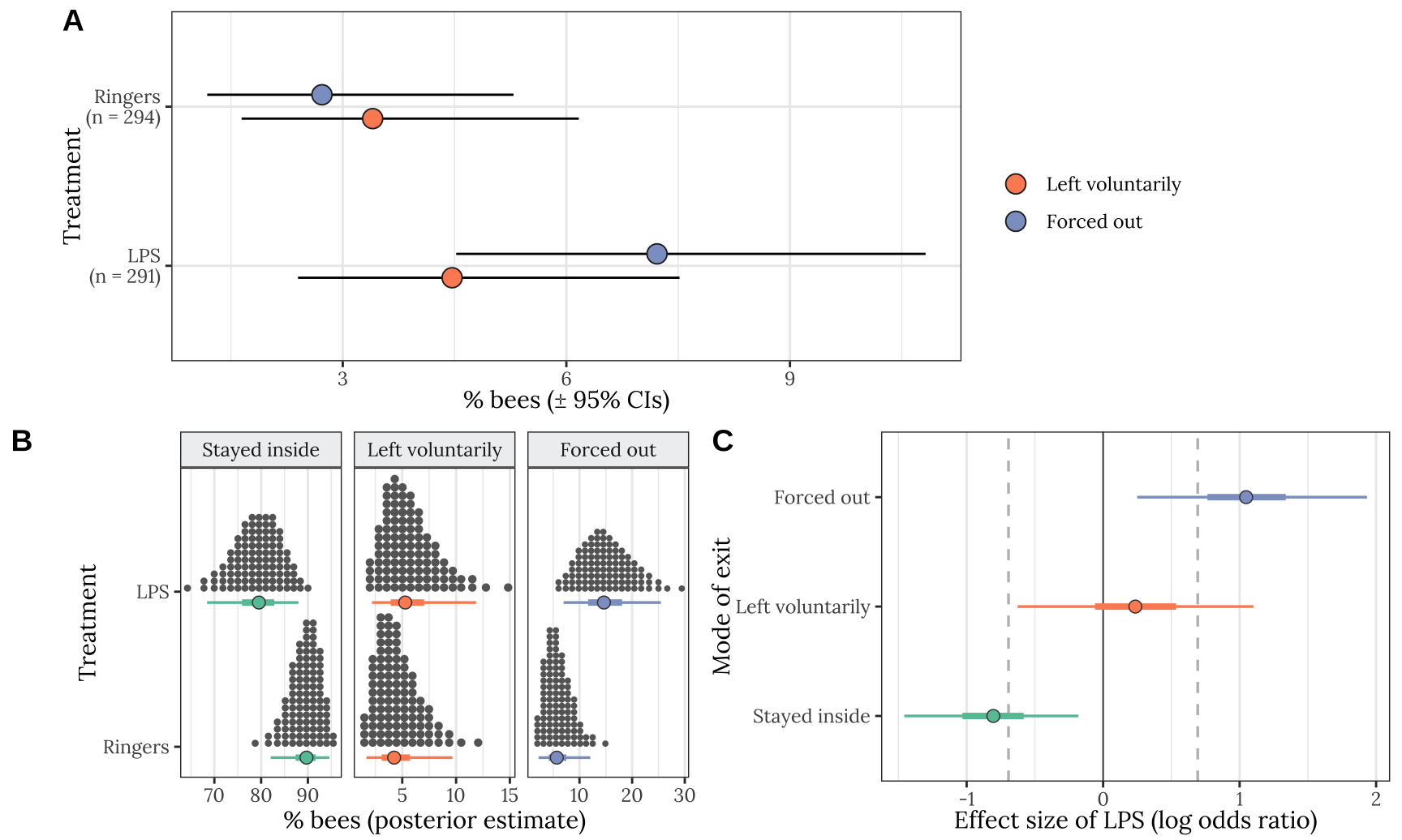
Figure 2: Results of Experiment 2 (n = 585 bees). Panels A-B display the same information as the corresponding panels in Figure 1. Panel C gives the posterior estimates of the effect size (log odds ratio) of the LPS treatment as a log odds ratio, for each of the three possible outcomes; the details are the same as for Figure 1C.
Hypothesis testing and effect sizes
Posterior effect size estimates
This section calculates the effect size and 95% CIs that are shown in Figure 2B (and creates Table S4).
Table S4: This table gives statistics associated with each of the contrasts plotted in Figure 2B. Each pair of rows gives the absolute (i.e. the difference in % bees) and standardised effect size (as log odds ratio; LOR) for the LPS treatment, relative to the Ringers control, for one of the three possible outcomes (Stayed inside, Left voluntarily, or Forced out). A LOR of \(|log(x)|\) indicates that the outcome is \(x\) times more frequent in one treatment compared to the other, e.g. \(log(2) = 0.69\) indicates a two-fold difference in frequency. The \(PP\) column gives the posterior probability that the true effect size has the same sign as is shown in the Estimate column; this metric has a similar interpretation to a one-tailed \(p\) value in frequentist statistics.
my_summary <- function(df, columns, outcome) {
  lapply(columns, function(x){

    p <- 1 - (df %>% pull(!! x) %>%
                bayestestR::p_direction() %>% as.numeric())

    df %>% pull(!! x) %>% posterior_summary() %>% as_tibble() %>%
      mutate(PP = p, Outcome = outcome, Metric = x) %>%
      select(Outcome, Metric, everything())
  }) %>% do.call("rbind", .)
}

stats_table <- rbind(
  plotting_data %>%
    filter(outcome == "Stayed inside") %>%
    spread(treatment, prop) %>%
    mutate(`Absolute difference in % bees staying inside` = 100 * (LPS - Ringers),
           `Log odds ratio` = get_log_odds(Ringers, LPS)) %>%
    my_summary(c("Absolute difference in % bees staying inside",
                 "Log odds ratio"),
               outcome = "Stayed inside") %>%
    mutate(PP = c(" ", format(round(PP[2], 4), nsmall = 4))),

  plotting_data %>%
    filter(outcome == "Left voluntarily") %>%
    spread(treatment, prop) %>%
    mutate(`Absolute difference in % bees leaving voluntarily` = 100 * (LPS - Ringers),
           `Log odds ratio` = get_log_odds(Ringers, LPS)) %>%
    my_summary(c("Absolute difference in % bees leaving voluntarily",
                 "Log odds ratio"),
               outcome = "Left voluntarily") %>%
    mutate(PP = c(" ", format(round(PP[2], 4), nsmall = 4))),

  plotting_data %>%
    filter(outcome == "Forced out") %>%
    spread(treatment, prop) %>%
    mutate(`Absolute difference in % bees forced out` = 100 * (LPS - Ringers),
           `Log odds ratio` = get_log_odds(Ringers, LPS)) %>%
    my_summary(c("Absolute difference in % bees forced out",
                 "Log odds ratio"),
               outcome = "Forced out") %>%
    mutate(PP = c(" ", format(round(PP[2], 4), nsmall = 4)))
) %>%
  mutate(` ` = ifelse(PP < 0.05, "\\*", ""),
         ` ` = replace(` `, PP < 0.01, "**"),
         ` ` = replace(` `, PP < 0.001, "***"),
         ` ` = replace(` `, PP == " ", ""))

stats_table[c(2,4,6), 1] <- " "

stats_table %>%
  select(-Outcome) %>% saveRDS("figures/tableS4.rds")


stats_table %>%
  select(-Outcome) %>%
  kable(digits = 3) %>% kable_styling(full_width = FALSE) %>%
  row_spec(c(0,2,4,6), extra_css = "border-bottom: solid;") %>%
  pack_rows("% bees staying inside", 1, 2) %>%
  pack_rows("% bees leaving voluntarily", 3, 4) %>%
pack_rows("% bees forced out", 5, 6)| Metric | Estimate | Est.Error | Q2.5 | Q97.5 | PP | |
|---|---|---|---|---|---|---|
| % bees staying inside | ||||||
| Absolute difference in % bees staying inside | -10.159 | 4.450 | -19.538 | -2.191 | ||
| Log odds ratio | -0.808 | 0.328 | -1.457 | -0.181 | 0.0051 | ** |
| % bees leaving voluntarily | ||||||
| Absolute difference in % bees leaving voluntarily | 1.122 | 2.234 | -3.060 | 5.922 | ||
| Log odds ratio | 0.238 | 0.442 | -0.627 | 1.101 | 0.2953 | |
| % bees forced out | ||||||
| Absolute difference in % bees forced out | 9.037 | 4.205 | 1.959 | 18.298 | ||
| Log odds ratio | 1.057 | 0.430 | 0.250 | 1.933 | 0.0053 | ** |
sessionInfo()R version 4.0.3 (2020-10-10)
Platform: x86_64-apple-darwin17.0 (64-bit)
Running under: macOS Catalina 10.15.7
Matrix products: default
BLAS: /Library/Frameworks/R.framework/Versions/4.0/Resources/lib/libRblas.dylib
LAPACK: /Library/Frameworks/R.framework/Versions/4.0/Resources/lib/libRlapack.dylib
locale:
[1] en_GB.UTF-8/en_GB.UTF-8/en_GB.UTF-8/C/en_GB.UTF-8/en_GB.UTF-8
attached base packages:
[1] stats graphics grDevices utils datasets methods base
other attached packages:
[1] car_3.0-8 carData_3.0-4 cowplot_1.0.0 tidybayes_2.0.3 bayestestR_0.11.5 kableExtra_1.3.4
[7] gridExtra_2.3 forcats_0.5.0 stringr_1.4.0 dplyr_1.0.0 purrr_0.3.4 readr_2.0.0
[13] tidyr_1.1.0 tibble_3.0.1 ggplot2_3.3.2 tidyverse_1.3.0 bayesplot_1.7.2 lme4_1.1-23
[19] Matrix_1.2-18 brms_2.14.4 Rcpp_1.0.4.6 showtext_0.9-2 showtextdb_3.0 sysfonts_0.8.3
[25] workflowr_1.6.2
loaded via a namespace (and not attached):
[1] readxl_1.3.1 backports_1.1.7 systemfonts_0.2.2 plyr_1.8.6 igraph_1.2.5
[6] svUnit_1.0.3 splines_4.0.3 crosstalk_1.1.0.1 TH.data_1.0-10 rstantools_2.1.1
[11] inline_0.3.15 digest_0.6.25 htmltools_0.5.0 rsconnect_0.8.16 fansi_0.4.1
[16] magrittr_2.0.1 openxlsx_4.1.5 tzdb_0.1.2 modelr_0.1.8 RcppParallel_5.0.1
[21] matrixStats_0.56.0 vroom_1.5.3 svglite_1.2.3 xts_0.12-0 sandwich_2.5-1
[26] prettyunits_1.1.1 colorspace_1.4-1 blob_1.2.1 rvest_0.3.5 haven_2.3.1
[31] xfun_0.26 callr_3.4.3 crayon_1.3.4 jsonlite_1.7.0 survival_3.2-7
[36] zoo_1.8-8 glue_1.4.2 gtable_0.3.0 emmeans_1.4.7 webshot_0.5.2
[41] V8_3.4.0 pkgbuild_1.0.8 rstan_2.21.2 abind_1.4-5 scales_1.1.1
[46] mvtnorm_1.1-0 DBI_1.1.0 miniUI_0.1.1.1 viridisLite_0.3.0 xtable_1.8-4
[51] bit_1.1-15.2 foreign_0.8-80 stats4_4.0.3 StanHeaders_2.21.0-3 DT_0.13
[56] datawizard_0.2.1 htmlwidgets_1.5.1 httr_1.4.1 threejs_0.3.3 RColorBrewer_1.1-2
[61] arrayhelpers_1.1-0 ellipsis_0.3.1 farver_2.0.3 pkgconfig_2.0.3 loo_2.3.1
[66] dbplyr_1.4.4 labeling_0.3 tidyselect_1.1.0 rlang_0.4.6 reshape2_1.4.4
[71] later_1.0.0 munsell_0.5.0 cellranger_1.1.0 tools_4.0.3 cli_2.0.2
[76] generics_0.0.2 broom_0.5.6 ggridges_0.5.2 evaluate_0.14 fastmap_1.0.1
[81] yaml_2.2.1 bit64_0.9-7 processx_3.4.2 knitr_1.32 fs_1.4.1
[86] zip_2.1.1 nlme_3.1-149 whisker_0.4 mime_0.9 projpred_2.0.2
[91] xml2_1.3.2 rstudioapi_0.11 compiler_4.0.3 shinythemes_1.1.2 curl_4.3
[96] gamm4_0.2-6 reprex_0.3.0 statmod_1.4.34 stringi_1.5.3 highr_0.8
[101] ps_1.3.3 Brobdingnag_1.2-6 gdtools_0.2.2 lattice_0.20-41 nloptr_1.2.2.1
[106] markdown_1.1 shinyjs_1.1 vctrs_0.3.0 pillar_1.4.4 lifecycle_0.2.0
[111] jquerylib_0.1.1 bridgesampling_1.0-0 estimability_1.3 data.table_1.12.8 insight_0.14.5
[116] httpuv_1.5.3.1 R6_2.4.1 promises_1.1.0 rio_0.5.16 codetools_0.2-16
[121] boot_1.3-25 colourpicker_1.0 MASS_7.3-53 gtools_3.8.2 assertthat_0.2.1
[126] rprojroot_1.3-2 withr_2.2.0 shinystan_2.5.0 multcomp_1.4-13 mgcv_1.8-33
[131] parallel_4.0.3 hms_0.5.3 grid_4.0.3 coda_0.19-3 minqa_1.2.4
[136] rmarkdown_2.11 git2r_0.27.1 shiny_1.4.0.2 lubridate_1.7.10 base64enc_0.1-3
[141] dygraphs_1.1.1.6